Kane’s Method for Dynamics

This page summarizes/motivates how Kane’s dynamical equations of motion are derived and used. Basic understanding of vector mechanics and derivatives is assumed.

There are a few references I have used when preparing these notes, but the clearest was this thesis.

Review of Lagrange’s Equations:

The steps in Lagranges equations are:

1. Let $\bm{r}_i$ be the location of the $i$-th particle in an inertial frame. Express this position as a function of a set of generalized coordinates:

$$\bm{r}_i = \bm{r_i}(q_1, ... q_{(3N-k)})$$

where $N$ is the number of particles in the system, $3N$ because each particle has a 3d coordinate, and $-k$ because there might be $k$ configuration constraints. So overall, we need $3N-k$ scalar quantities (degrees of freedom) to uniquely define the configuration of the system.

1. Determine the Lagrangian:

$$L = T - U$$

where $T(q_1, ... , q_{3N-k}, \dot q_1, ..., \dot q_{3N-k})$ is the kinetic energy of the system, and $U(q_1, ... , q_{3N-k})$ is the potential energy of the system.

1. Then the equations of motion are:

$$\frac{d}{dt}\left(\frac{\partial L}{\partial \dot{q}_i}\right) - \frac{\partial L}{\partial q_i} = Q_i, \quad i=\{1, ... , 3N-k\}$$

where

$$Q_i = \sum_{j=1}^{N} \bm{F}_j \cdot \frac{\partial \bm{r}_j}{\partial q_i}$$

is the contribution of non-conservative/external forces.

Notice, we will have generated $3N-k$ 2nd order equations. If there are non-holonomic constraints, these are usually introduced as additional constraint equations, with lagrange multipliers. (I’ll explain this better once I understand it myself).

Derivation of Kane’s method (for system of particles)

Kanes method is basically a souped-up version of Newton’s 2nd law/D’Alemberts principle:

$$\bm{R}^{P_i} - m^{P_i} \bm{a}^{P_i} = 0, \quad i = \{1, ... \nu\}$$

where

• $\bm{R}^{P_i}$ is the net force on the $i$-th particle
• $m^{P_i}$ is the mass of the $i$-th particle
• $\bm{a}^{P_i}$ is the acceleration of the $i$-th particle
• $\nu$ is the number of particles.

Now suppose the position/configuration of the system can be uniquely described by a set of $p$ scalar coefficients (and potentially time):

$$\bm {r}^{P_i} = \bm{r}^{P_i}(q_1, ..., q_p, t)$$

then the velocity in some inertial frame is

$$\bm{v}^{P_i} = \frac{d \bm{r}^{P_i} }{dt} = \sum_{r=1}^{p} \frac{\partial \bm{r}^{P_i}}{\partial q_r} \dot q_r + \frac{\partial \bm{r}^{P_i}}{\partial t}$$

Often, we can simplify this expression by choosing a convenient set of generalised speeds $u_i$. In Lagranges formulation, the generalised speeds $u_r = \dot q_r$. However, we can be more general, allowing functions of $q, \dot q$:

$$u_r = u_r(q_1, ..., q_p, \dot{q}_1, ..., \dot{q}_p), \quad r = \{1, ..., p\}$$

and we need $p$ generalised speeds, so that this map is invertible (to be able to find $\dot q_i$ in terms of $u$). This allows us to write

$$\bm{v}^{P_i} = \sum_{r=1}^{p} \bm{v}_r^{P_i} u_r + \bm{v}_t^{P_i}$$

where

$$\bm{v}_r^{P_i} = \frac{\partial \bm{v}^{P_i}}{\partial u_r}, \quad \bm{v}_t^{P_i} = \frac{\partial \bm{v}^{P_i}}{\partial t}$$

If there $s$ non-holonomic constraints, we rearrange the variables such that last $s$ generalised speeds can be represented as linear combinations of the first $p-s$ generalised speeds. Then, we can also write

$$\bm{v}^{P_i} = \sum_{r=1}^{p-s} \tilde{\bm{v}}_r^{P_i} u_r + \tilde{\bm{v}}_t^{P_i}$$

where

$$\tilde{\bm{v}}_r^{P_i} = \frac{\partial \bm{v}^{P_i}}{\partial u_r}, \quad \tilde{\bm{v}}_t^{P_i} = \frac{\partial \bm{v}^{P_i}}{\partial t}$$

where we have expressed $\bm{v}$ only in terms of the first $p-s$ generalised speeds, $u_r$.

Now we return to Newton’s equation:

$$\bm{R}^{P_i} - m^{P_i} \bm{a}^{P_i} = 0, \quad i = \{1, ... \nu\}$$

and notice that if we take the dot product of this equation with $\tilde{\bm{v}}_r$, we get

$$\tilde{\bm{v}}_r^{P_i} \cdot \bm{R}^{P_i} - m^{P_i} \tilde{\bm{v}}_r^{P_i} \cdot \bm{a}^{P_i} = 0, \quad i = \{1, ... \nu\}$$

and now we can sum across all particles, giving us an equation for each generalised speed, rather than for each particle in the system!

$$\boxed{ \underbrace{\sum_{i=1}^{\nu} \tilde{\bm{v}}_r^{P_i} \cdot \bm{R}^{P_i}}_{F_r} + \underbrace{\sum_{i=1}^{\nu} -m^{P_i} \tilde{\bm{v}}_r^{P_i} \cdot \bm{a}^{P_i}}_{F_r^*} = 0, }\quad r = \{1, ..., p-s\}$$

which gives $p-s$ equations of motion, called Kane’s Dynamical Equations of Motion.

Kane’s Method for Bodies

The same general method is used, but we also need to introduce equations that describe the rotational dynamics of the system.

If a rigid body B belongs to a non-holonomic system S with $p$ degrees of freedom in an inertial reference frame A, the set of all forces and torques on B can be summarised by a single resultant force $\bm R^{B}$ acting through a point $Q$ of B, and a torque $\bm T$ on B. Then the generalised active force is

$$\tilde F_r^{B} = {}^A \tilde{\bm{\omega}}_r^{B} \cdot \bm T + \tilde{\bm{v}}_r^{Q} \cdot \bm{R}^B, \quad r=\{1, ..., p\}$$

and the inertial forces are:

$$\tilde {F_r^{B}}^* = {}^A \tilde{\bm{\omega}}_r^{B} \cdot \bm T^* + \tilde{\bm{v}}_r^{Q} \cdot {\bm{R}^*}^B, \quad r=\{1, ..., p\}$$

where

$$\begin{align*} {\bm{R}^*}^B &= -m^B \bm{a}^*\\ \bm T^* &= - \bm \alpha \cdot \bm I - \bm \omega \times \bm I \cdot \bm \omega = - \sum_{i=1}^{\beta} m_i \bm r_i \times \bm a_i \end{align*}$$

where $\bm a^*$ is the acceleration of the center of mass of B in A, and if there are $\beta$ individual particles in B, the second version of $T^*$ can be used, or if the central inertia dyadic of B is known, the first version of $T^*$ can be used. If the principal central moments of inertia are known, and are aligned with a frame C, we can also write:

$$\begin{align*} \bm T^* = &- (\alpha_1 I_1 - \omega_2 \omega_3 (I_2 - I_3)) \bm c_1 \\ & - (\alpha_2 I_2 - \omega_3 \omega_1 (I_3 - I_1)) \bm c_2 \\ & - (\alpha_3 I_3 - \omega_1 \omega_2 (I_1 - I_2)) \bm c_3 \end{align*}$$

where $\bm \alpha = \alpha_1 \bm c_1 + \alpha_2 \bm c_2 + \alpha_3 \bm c_3$, and ${}^N \bm \omega^B = \omega_1 \bm c_1 + \omega_2 \bm c_2 + \omega_3 \bm c_3$

Finally, the dynamical equations of motion are

$$\sum_{i=1}^{\nu} \tilde F_r^{B_i} + {\tilde F_r^{B_i}}^* = 0, \quad r=\{1, ..., p\}$$

for each of the $\nu$ bodies in the system. Together with the kinematic differential equations $\dot q_r = \dot q_r(q, u)$, the equations of motion are complete.

---

Example 1: Spring Pendulum

Consider this problem, taken from the reference above.

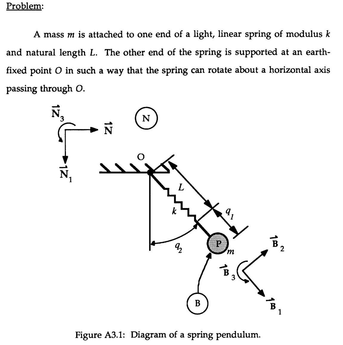
The position of the particle is

$$\bm r^{P_1} = (L+ q_1) \bm b_1$$

and so the velocity in the inertial frame $N$ is

$$\bm v^{P_1} = \dot q_1 \bm b_1 + {}^N\bm{\omega}^B \times (L+q_1) \bm b_1 = \dot q_1 \bm b_1 + (L+q_1)\dot q_2 \bm b_2$$

which motivates the definition of generalised speeds:

$$u_1 = \dot q_1, \quad u_2 = (L+q_1) \dot q_2$$

and so $\bm v^{P_1} = u_1 \bm b_1 + u_2 \bm b_2$. Thus the partial velocities are

$$\bm v_1^{P_1} = \bm b_1, \quad \bm v_2^{P_2} = \bm b_2$$

and we can compute the acceleration of particle 1:

$$\begin{align*} \bm a^{P_1} &= \dot u_1 \bm b_1 + \dot u_2 \bm b_2 + u_1 {}^N \bm{\omega}^B \times \bm b_1 + u_2 {}^N \bm{\omega}^B \times \bm b_2 \\ &= \dot u_1 \bm b_1 + \dot u_2 \bm b_2 + u_1 \dot q_2 \bm b_2 - u_2 \dot q_2 \bm b_1\\ &= \dot u_1 \bm b_1 + \dot u_2 \bm b_2 + \left(\frac{u_1 u_2}{L+q_1}\right) \bm b_2 - \left(\frac{u_2^2}{L+q_1}\right) \bm b_1\\ \therefore \bm a^{P_1} &= \bm b_1 \left( \dot u_1 - \frac{u_2^2}{L+q_1} \right) + \bm b_2 \left( \dot u_2 + \frac{u_1 u_2}{L+q_1}\right) \end{align*}$$

Lets now find the forces on the particle:

$$\bm{R}^{P_1} = mg \bm n_1 - k q_1 \bm b_1$$

and so we are almost ready to write Kanes equations of motion. Lets find $F_r$ and then $F_r^*$:

$$F_r = \sum_{i=1}^{\nu} \tilde{\bm{v}}_r^{P_i} \cdot \bm{R}^{P_i}$$

Since we have one particle $\nu = 1$ and 2 generalised speeds $r = \{ 1, 2 \}$. So

$$\begin{align*} F_1 &= \tilde{\bm{v}}_1^{P_1} \cdot \bm{R}^{P_1}\\ &= \bm b_1 \cdot (mg \bm n_1 - k q_1 \bm b_1)\\ &= mg \cos q_2 - k q_1\\ F_2 &= \tilde{\bm{v}}_2^{P_1} \cdot \bm{R}^{P_1}\\ &= \bm b_2 \cdot (mg \bm n_1 - k q_1 \bm b_1)\\ &= -mg \sin q_2 \end{align*}$$

and

$$F_r^* = \sum_{i=1}^{\nu} \tilde{\bm{v}}_r^{P_i} \cdot (-m^{P_i} \bm a^{P_i})$$

so

$$\begin{align*} F_1^* &= \tilde{\bm{v}}_1^{P_1} \cdot (-m^{P_1} \bm a^{P_1})\\ &= \bm b_1 \cdot (-m) \left( \bm b_1 \left( \dot u_1 - \frac{u_2^2}{L+q_1} \right) + \bm b_2 \left( \dot u_2 + \frac{u_1 u_2}{L+q_1}\right)\right)\\ &= -m \left( \dot u_1 - \frac{u_2^2}{L+q_1} \right)\\ F_2^* &= \tilde{\bm{v}}_2^{P_1} \cdot (-m^{P_1} \bm a^{P_1})\\ &= \bm b_2 \cdot (-m) \left( \bm b_1 \left( \dot u_1 - \frac{u_2^2}{L+q_1} \right) + \bm b_2 \left( \dot u_2 + \frac{u_1 u_2}{L+q_1}\right)\right)\\ &= -m \left( \dot u_2 + \frac{u_1 u_2}{L+q_1} \right) \end{align*}$$

and so putting it together,

$$\begin{align*} F_1 + F_1^* = mg \cos q_2 - k q_1 -m \left( \dot u_1 - \frac{u_2^2}{L+q_1} \right) &= 0\\ F_2 + F_2^* = -mg \sin q_2 -m \left( \dot u_2 + \frac{u_1 u_2}{L+q_1} \right) &= 0 \end{align*}$$

which means that the kinematic (first two) and dynamical (last two) equations that describe this system are:

$$\boxed{ \begin{align*} \dot q_1 &= u_1\\ \dot q_2 &= \frac{u_2}{L+q_1} \\ \dot u_1 &= g \cos q_2 - (k/m) q_1 + \frac{u_2^2}{L+q_1}\\ \dot u_2 &= -g \sin q_2 - \frac{u_1 u_2}{L+q_1} \end{align*} }$$

Example 2: Hinged Rods