Nonlinear Observers

This tech note summarizes the design of Nonlinear Observers, based on LMI conditions from this seminar, by Rajesh Rajamani.

TLDR:

For the nonlinear system

\[\begin{align} \dot x &= A x + f(x)\\ y &= Cx \end{align}\]

with state \(x\), measurements \(y\) and Lipschitz continuous function \(f\) with Lipschitz constant \(\gamma\). The estimated state is \(\hat x\) with dynamics

\[\begin{align} \dot{\hat x} = A\hat x + f(\hat x) + L ( y - C \hat x) \end{align}\]

where \(L\) is the observer gain matrix.

To find \(L\), we solve the Linear Matrix Inequality (LMI):

\[\begin{align} \text{find} \quad & \alpha, P, R\\ \text{subject to} \quad & \begin{bmatrix} PA + A^T P - RC - C^T R^T + \gamma^2 I+ \alpha P & P \\ P & -I \end{bmatrix} \leq 0\\ &P > 0\\ & \alpha \geq 0\\ & e_0^T P e_0 = 1 \end{align}\]

over the variables \(\alpha, P, R\). The observer gains are

\[L = P^{-1} R\]

This guarantees an error convergence rate of \(\alpha\) for the Lyapunov function \(V = e^T P e\) (ie. convergence rate of $2\alpha$ for \(\Vert e\Vert\)), where \(e = x - \hat x\), if a solution to the optimization problem can be found.

---

Set up:

System

We will consider nonlinear systems of the form

\[\begin{align} \dot x &= A x + f(x)\\ y &= Cx \end{align}\]

where \(x \in \mathbb{R}^n\) is the state, and \(y \in \mathbb{R}^p\) is the measurement. \(A, C\) are constant real matrices, and \(f(x)\) is a nonlinearity, which we will assume is Lipschitz continuous with constant \(\gamma\):

\[\left\Vert f(x) - f(y) \right \Vert \leq \gamma \left \Vert x-y \right \Vert\]

for all \(x, y\).

Observer Form

The observer will be of the form

\[\begin{align} \dot{\hat x} = A\hat x + f(\hat x) + L ( y - C \hat x) \end{align}\]

where \(\hat x\) is the estimated state, and \(L\) is the observer gain matrix that we need to design.

The objective is to design \(L\) such that the error \(x - \hat x \to 0\) as \(t \to \infty\).

Observer Error Dynamics

Let the estimation error be

\[\begin{align} e = x - \hat x \end{align}\]

the dynamics of \(e\) are

\[\begin{align} \dot e &= \dot x - \dot{ \hat x}\\ &= \left[ A x + f(x) \right] - \left[ A\hat x + f(\hat x) + L (C x - C \hat x) \right]\\ &= (A - LC )e + f(x) - f(\hat x) \end{align}\]

Notice that if the system was linear (\(f(x) = 0\)), then we are done: we just need \(A-LC\) to be a Hurwitz matrix, and we would have proved that the error dynamics are exponentially stable.

We introduce the basic version of designing \(L\), and then demonstrate a few extensions.

Design:

Consider a Lyapunov function

\[\begin{align} V(e) = e^T P e \end{align}\]

where \(P\) is a symmetric positive definite matrix. The derivative of \(V\) is

\[\begin{align} \dot V &= e^T P \dot e + \dot e^T P^T e\\ &= e^T (P (A-LC) + (A-LC)^T P)e + \tilde{f}^T P e + e^T P \tilde{f} \end{align}\]

where we used the notation \(\tilde f = f(x) - f(\hat x)\). Now we can use the Lipschitz constant to bound \(\dot V\):

\[\begin{align} \dot V &\leq e^T (P (A-LC) + (A-LC)^T P)e + (\gamma \Vert e \Vert) \Vert P e \Vert + \Vert e^T P \Vert (\gamma \Vert e \Vert)\\ &= e^T (P (A-LC) + (A-LC)^T P)e + 2 \gamma \Vert P e \Vert \Vert e \Vert\\ &\leq e^T (P (A-LC) + (A-LC)^T P)e + \gamma^2 \Vert e \Vert^2 + \Vert P e \Vert^2\\ &= e^T \left [ P (A-LC) + (A-LC)^T P + \gamma^2 I + P P \right] e \\ \end{align}\]

where to go from the 2nd to 3rd step, we used the rule \(2 a b \leq a^2 + b^2\).

Notice that in this form, we have bounded \(\dot V\) for the nonlinear error dynamics, in terms of the error \(e\) and independently of \(x, \hat x\).

Thus, all we need to do is to ensure the matrix on the inside is negative definite:

\[\begin{align} \therefore [ P (A-LC) + (A-LC)^T P + \gamma^2 I + P P ] < 0 \quad \implies e \to 0 \text{ as } t \to \infty \end{align}\]

We generalise this slightly, to the case where we a specific exponential convergence rate \(\alpha\). Thus, we want \(\dot V \leq - \alpha V\). Thus, we want

\[\begin{align} [ P (A-LC) + (A-LC)^T P + \gamma^2 I + P P ] \leq - \alpha P \end{align}\]

for some \(\alpha \geq 0\). Notice that if \(\alpha = 0\), we will know that the error dynamics are stable, not necessarily asymptotically or exponentially stable.

The objective is now to determine \(P, L\) such that the above holds. As we will show later, we could also let \(\alpha\) be an decision variable, and try to find \(P\), \(L\) such that \(\alpha\) is as large as possible, ie for the greatest convergence rate.

We can write this condition as a Linear Matrix Inequality (LMI). See Boyd’s books on LMIs or Convex Optimization for a explanation of LMIs.

Unfortunately, the condition above involves products of matrices, specifically \(PL\) and \(PP\). We can remedy this using two tricks:

TRICK 1: Define \(R = PL\).

and now \(P, R\) are the decision variable, instead of \(P, L\). The condition is

\[[ PA + A^T P - RC - C^T R^T + \gamma^2 I + P P + \alpha P ] \leq 0\]

and now the problem is linear in \(R\).

TRICK 2: Schur Complements

Using the schur complement trick, we can write the above condition as

\[Q = \begin{bmatrix} PA + A^T P - RC - C^T R^T + \gamma^2 I+ \alpha P & P \\ P & -I \end{bmatrix} \leq 0\]

which looks like a mess, but is now linear in \(P\) and \(R\). We define this matrix as \(Q\) for convenience.

We can solve this LMI, using tools like Convex.jl and SCS (open source) (see below for code):

\[\begin{align} \text{find} \quad & \alpha, P, R\\ \text{subject to} \quad & Q \leq 0\\ &P > 0\\ & \alpha \geq 0\\ & e_0^T P e_0 = 1 \end{align}\]

where the last condition is used to normalise \(P\): we require the value of \(V\) at \(e_0 = [1, 0, ..., 0]^T\) to be 1.

Finally, we can determine the observer gains:

\[L = P^{-1} R\]

which is always possible, since \(P\) is a positive definite matrix (assuming a solution to the optimization problem was found).

Extensions:

Refer to the seminar video for more details.

Extension 1: Modified Lipschitz bound

We can consider a modified Lipschitz bound, of the form

\[\Vert f(x) - f(\hat x) \Vert \leq \Vert G (x - \hat x) \Vert\]

where \(G\) is a constant matrix. Following the steps from above, we can re-write \(Q\) as

\[Q = \begin{bmatrix} PA + A^T P - RC - C^T R^T + G^T G+ \alpha P & P \\ P & -I \end{bmatrix} \leq 0\]

which can be less conservative. Essentially, we have replaced \(\gamma^2 I\) with \(G^T G\). If \(G\) is sparse, this can be a useful improvement.

The rest of the steps are identical.

Extension 2: Bounded Gradients

If, instead of the Lipschitz constant condition, we have

\[K_1 \leq \frac{df}{dx} \leq K_2\]

for some matrices \(K_1, K_2\), we can show that (by the mean value theorem)

\[(\tilde f - K_1 e )^T (\tilde f - K_2 e) \leq 0\]

then we can rewrite \(Q\):

\[Q = \begin{bmatrix} PA + A^T P - RC - C^T R^T + \alpha P & P \\ P & -I \end{bmatrix} + \frac{1}{2} \begin{bmatrix} M & N^T\\ N & 0 \end{bmatrix} \leq 0\]

where

\[M = -( K_1^T K_2 + K_2^T K_1) , \quad N = K_1 + K_2\]

The rest of the design process is the same as before.

Extension 3: Disturbance Rejection

Suppose the system also receives some disturbance \(w(t)\):

\[\begin{align} \dot x &= A x + f(x) + B w\\ y &= Cx \end{align}\]

For a \(\mathcal{H}_\infty\) disturbance rejection requirement \(\mu > 0\):

\[\int_0^\infty e^T e dt \leq \mu \int_0^\infty w^T w dt\]

we modify \(Q\) to

\[Q = \begin{bmatrix} PA + A^T P - RC - C^T R^T + G^TG + \alpha P & P & PB \\ P & -I & 0\\ B^T P & 0 & - \mu I \end{bmatrix} \leq 0\]

The rest of the design process is the same as before.

Extension 4: Bilinear Optimization

Suppose we wish to make \(\alpha\) as large as possible. We can do this, by performing a bi-linear optimization. We solve the optimization

\[\begin{align} \text{maximise} \quad & \alpha\\ \text{subject to} \quad & Q \leq 0\\ &P > 0\\ & \alpha \geq 0\\ & e_0^T P e_0 = 1 \end{align}\]

first by fixing \(\alpha\) freeing $P$, and then by fixing $P$ and freeing \(\alpha\).

Doing this maintains the linearity, and allows \(\alpha\) to grow.

Alternatively, one could do a simple line search to see which \(\alpha\) is the largest that can be reached. Be careful of numerical issues when \(\alpha\) gets large though!

---

Example:

Consider the nonlinear system

\[\begin{align} \dot x_1 &= x_2 - \sin x_1\\ \dot x_2 &= - x_1 - 2 x_2\\ y & = x_1 \end{align}\]

In standard form we have

\[\begin{align} \begin{bmatrix} \dot x_1 \\ \dot x_2\end{bmatrix} &= \begin{bmatrix} 0 & 1\\ -1 & -2 \end{bmatrix}x + \begin{bmatrix} \sin x_1\\ 0 \end{bmatrix}\\ y &= \begin{bmatrix} 1 & 0 \end{bmatrix} x \end{align}\]

Thus, the Lipschitz-type bound is

\[\begin{align} \Vert f(x_1) - f(x_2) \Vert &\leq \Vert G (x_1 - x_2) \Vert\\ \left \Vert \begin{bmatrix} \sin x_{1, 1}\\ 0 \end{bmatrix} - \begin{bmatrix} \sin x_{1, 2}\\ 0 \end{bmatrix} \right \Vert &\leq \left \Vert \begin{bmatrix} 1 & 0 \\ 0 & 0 \end{bmatrix} \begin{bmatrix} x_{1,1} - x_{1, 2}\\ x_{2,1 } - x_{2,2} \end{bmatrix} \right \Vert \end{align}\]

The code below solves the optimization problem:

using Convex, SCS, LinearAlgebra

A = [0 1; 
    -1 -2.]

f(x) = [-sin(x[1]), 0.0]

C = zeros(1,2)
C[1] = 1.0

G = [1 0;
     0 0.0]

nx = 2 # number of states
np = 1 # number of observations

α = 1.0

P = Variable((nx, nx))
R = Variable((nx, np))

Q = [(P*A + A'*P - R*C - C'*R' + G'*G + α*P) P ; P -diagm(ones(nx))]

constraints = [
    P == P',
    eigmax(Q) <= 0.0
    eigmin(P) >= 0.0,
    P[1,1] == 1.0
];

prob = satisfy(constraints)

solve!(prob, SCS.Optimizer)

@show P.value

@show R.value

L = inv(P.value) * (R.value)

@show L

This gave the result

\[P = \begin{bmatrix} 0.9999 & -0.0030\\ -0.0030 & 0.3146 \end{bmatrix}\] \[R = \begin{bmatrix} 2.40541\\ 0.69388 \end{bmatrix}\]

and thus, the observer gains are

\[L = \begin{bmatrix} 2.41216\\ 2.22836 \end{bmatrix}\]

We can also simulate this behaviour

using DifferentialEquations, Plots

function closedLoop(state, params, time)
    
    x = state[1:2]
    x̂ = state[3:4]

    # make a measurement
    y = C * x
    
    # propagate true state
    dx = A * x + f(x)

    # propagate estimated state
    dx̂ = A * x̂ + f(x̂) + L * (y - C * x̂)
  
    return vcat(dx, dx̂)
end

# define an random initial condition for the true state
# define (0,0) as the initial estimated state

x0 = [randn(2)..., 0, 0.]

# simulate for 10 seconds
tspan = (0, 10.)

# construct and solve the ODE problem
odeProb = ODEProblem(closedLoop, x0, tspan)
sol = solve(odeProb)

## Plots


plot(sol, vars=(0,1), label="True State x_1")
plot!(sol, vars=(0,2), label="True State x_2")
plot!(sol, vars=(0,3), linestyle=:dash, label="Estimated State x_1")
plot!(sol, vars=(0,4), linestyle=:dash, label="Estimated State x_2")
savefig("states.png")
plot!()



plot(t-> norm(sol(t)[1:2] - sol(t)[3:4]), tspan..., label="Norm(x-x̂)", xlabel="t")
savefig("norm_error.png")
plot!()

plot(t-> log(norm(sol(t)[1:2] - sol(t)[3:4])), tspan..., label="log(Norm(x-x̂))", xlabel="t")
plot!(t-> -2*α*t, tspan..., linestyle=:dash, label="Theoretical Convergence Rate")
savefig("log_norm_error.png")
plot!()

The plots are below

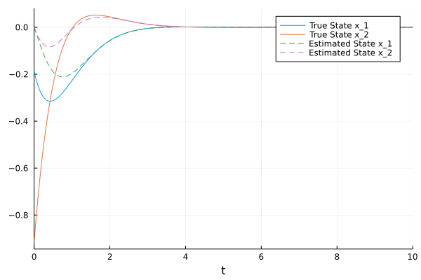
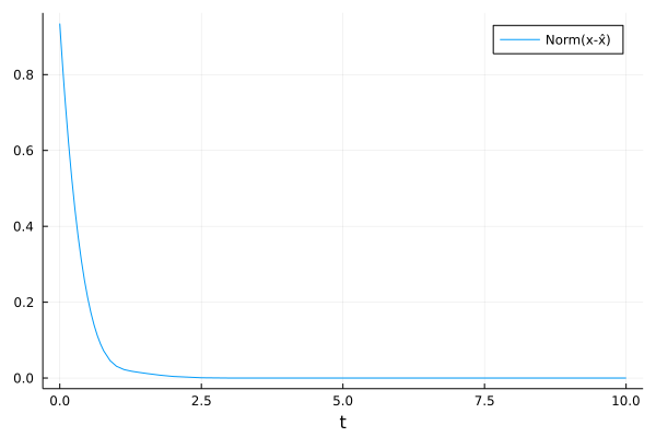
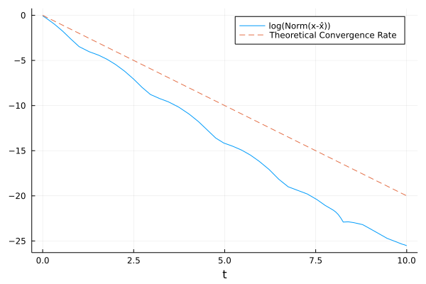
which shows that the estimation error converges to 0, slightly faster than expected.